Announcement

Collapse
No announcement yet.
X
  • Filter
  • Time
  • Show
Clear All
new posts

  • Anticipation Effect

    Hello, All.

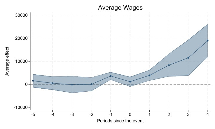
    I am working on Industry Survey data from 2003 to 2011. It is a repeated cross section. My treatment is staggered between 2006 and 2011. I apply a staggered DiD model (Callaway and Sant'Anna, 2020) using the csdid package in stata. My plot is attached below. There seems to be an issue with the pre trends. The policy was federally announced in 2005 however the first treatment took place in 2006, hence I assume the issue to be anticipation in period -1. This is making it tough for me to analyze the estimate computed. How should I proceed? What facts would help me infer causation? Is there a way to control for the anticipation effects? I do not have any covariates. Any advice is appreciated!


  • #2
    While what happened at time -1 may be an anticipation effect, it seems to be, if anything, larger than the effect seen at time 0. I'm no economist, but does that make sense? (Serious question.) If I were just presented with that graph and no specific context, the most obvious reading of it is that the system underwent some kind of state transition at time -1. While there was a little backsliding at time 0, that is easily within the range of random fluctuation for this system.

    Sure, you could revise your model a bit to treat time -1 as an anticipation period. But no matter what statistics that produces, you still have to explain why that is a better explanation for what happened than something important happening at time -1. No statistics can solve this problem for you: you will have to review the historical and economical context to convince your audience that there was no event at time -1 that could explain this. So step away from the keyboard and start hitting the history books.

    Comment


    • #3
      Clyde Schechter Thank you for your response. You are right, I will get to it!

      Comment


      • #4
        Something looks off to me in the graph. Isn't it typical to impose that the effect in period -1 is zero, and then all effects are measured relative to the period just before the intervention? That is the usual event study graph. That choice is essentially arbitrary, but one must choose one period before the intervention as the comparison period. This may be related to the fact that you have 9 years of data but have shown 10 estimated effects. With the intervention in 2006, the usual graph would show a zero effect (by construction) in 2005, and then the estimates for all other years would be relative to 2005.

        Because it was known in 2005 that the policy would go into effect in 2006, you could drop 2005 and start with 2004. Of course, this gives you only two pre-treatment periods, and so only one "pre-treatment" treatment effect (2003 to 2004).

        Comment


        • #5
          Another comment: Without covariates, Callaway and Sant'Anna is just the usual event study estimation, and so you should see what happens when you use standard event study commands. Or, just do the regression yourself.

          Comment


          • #6
            As Wooldridge pointed out, the fact that t -1 is also estimated (not set to 0) indicates that the model was estimated with the default option, which is the same in the R package.
            However, it is probably always better to use `long` or `long2` options. The pre-treatment trend will be probably much clearer.


            In the following link you can see a little deeper discussion on the issue and a comparison between the two options: https://github.com/friosavila/stpackages/issues/3


            Comment

            Working...
            X